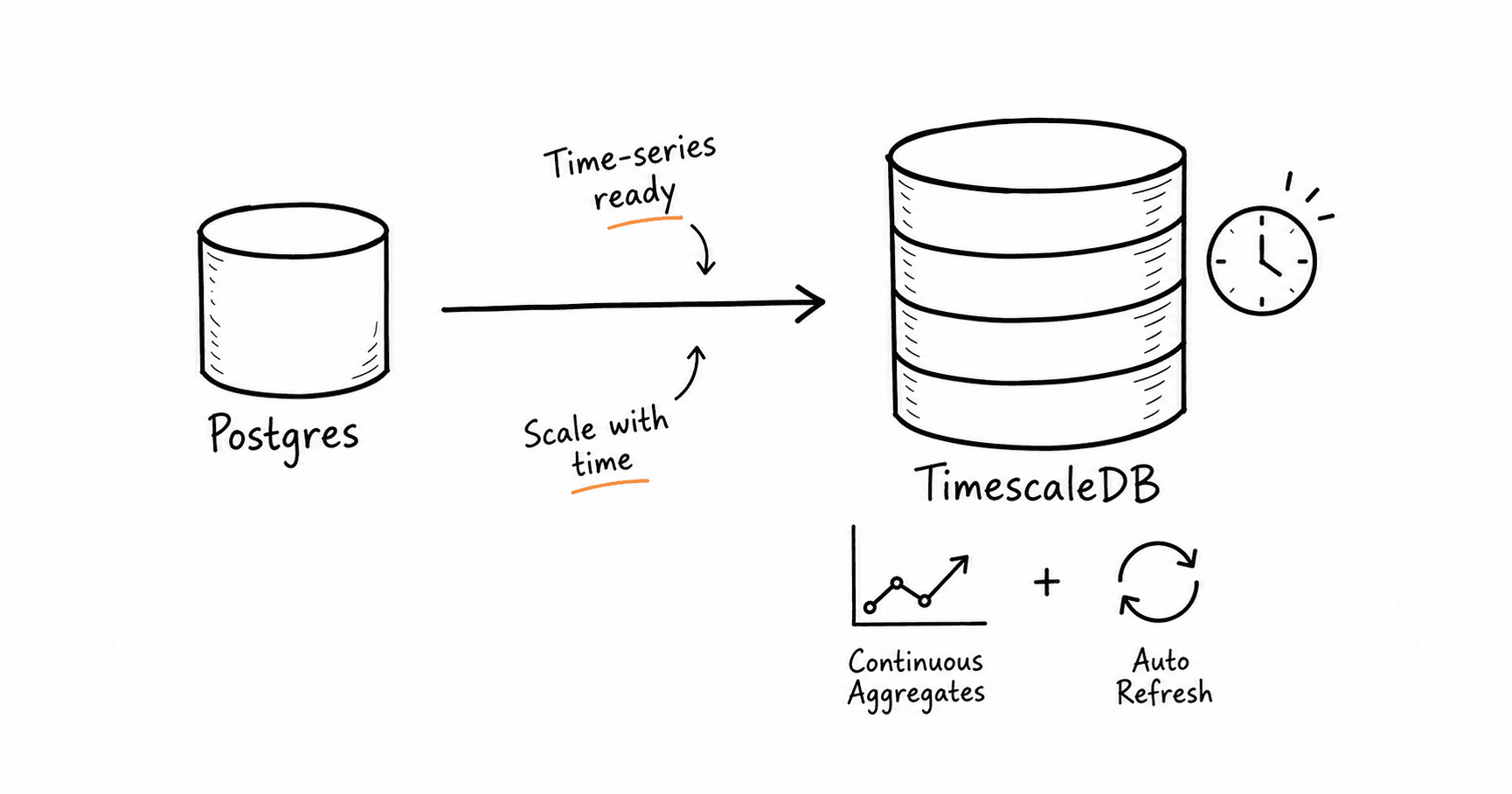
At some point, almost every growing application ends up with one table that quietly becomes a problem: a transaction log, an events table, a metrics table — something that's append-only, time-stamped, and growing by the day. Queries against it start fine and slowly get worse, until a dashboard that used to load instantly takes seconds, then tens of seconds.
This is the exact shape of problem TimescaleDB is built for. This post walks through setting it up end to end — from a Docker Compose container, through hypertables and compression, to continuous aggregates that keep themselves up to date on a schedule. I'll use a generic events table throughout as the running example, since the concepts matter more than any specific schema.
What TimescaleDB actually is
TimescaleDB is a PostgreSQL extension, not a separate database. You install it into a normal Postgres instance, and it adds features purpose-built for time-series data: automatic partitioning of large tables into smaller chunks, native compression for old data, and continuous aggregates — materialized views that update themselves incrementally instead of recomputing from scratch.
The important part is that it's still Postgres underneath. Your existing queries, tools, and mental model of joins and indexes don't change. What changes is how the data is physically organized and how efficiently time-range queries run against it.
Plain Postgres vs. TimescaleDB
A plain Postgres table with time-series data is stored as one continuous structure. As it grows, every operation — index maintenance, vacuuming, query planning — has to reason about the entire table, even if a given query only cares about the last week of data.
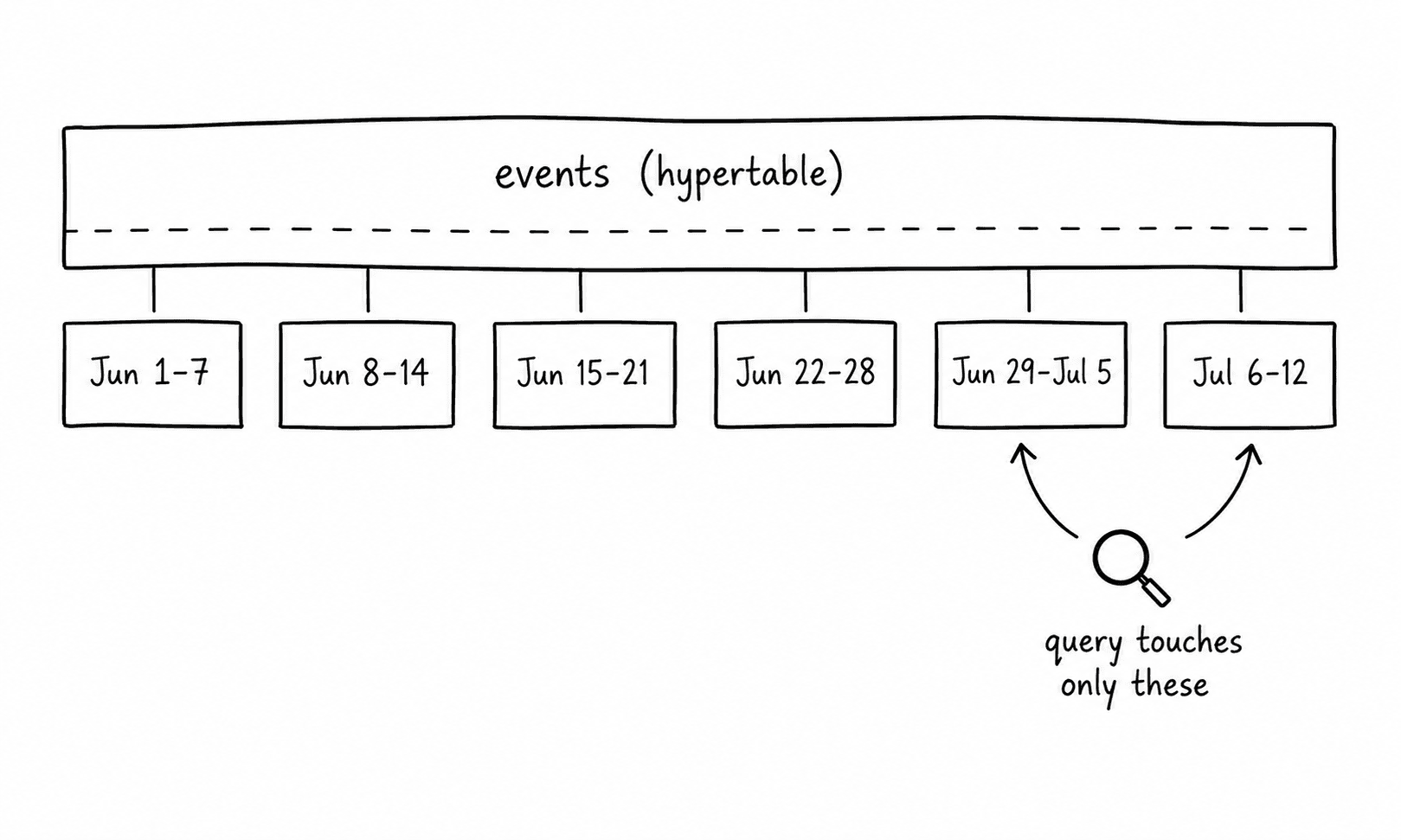
From the application's point of view, nothing looks different — you still INSERT and SELECT against one table called events. TimescaleDB is doing the partitioning underneath and routing queries to the right chunks automatically.
Why it's fast: how hypertables actually store data
A hypertable isn't really one table — it's a virtual view over many smaller physical tables, called chunks, each covering a fixed time interval. When you insert a row, TimescaleDB looks at its timestamp and routes it to the correct chunk, creating a new one automatically if needed.
- Smaller indexes per chunk. Each time range gets its own compact index, instead of one enormous index covering years of data.
- Query pruning. A query such as
WHERE created_at > now() - interval '1 day'skips every chunk outside that range entirely. - Cheaper maintenance. Vacuuming and reindexing operate per chunk, keeping maintenance proportional to active data rather than total history.
Pre-flight verification
Before converting an existing table into a hypertable, it's worth confirming a few things up front. Most failure modes here are avoidable with a five-minute check.
- Extension is installedConfirm TimescaleDB is active in the target database before running any hypertable commands.
SELECT default_version, installed_version FROM pg_available_extensions WHERE name = 'timescaledb'; - Primary key includes the time columnTimescaleDB requires the partitioning column to be part of the primary key. A non-time primary key needs to become composite.
- No NULLs in the time columnEvery row needs a valid timestamp to be routed into a chunk.
SELECT COUNT(*) FROM events WHERE created_at IS NULL; - Understand the data rangeCheck the minimum and maximum timestamps to estimate how many chunks the conversion will create.
SELECT MIN(created_at), MAX(created_at) FROM events; - Confirm it isn't already a hypertableUseful when re-running a migration or checking an unfamiliar table.
SELECT * FROM timescaledb_information.hypertables WHERE hypertable_name = 'events';
Creating a hypertable
If the table doesn't already have a primary key that includes the time column, add one first. This operation takes an exclusive lock, so on a production table it's worth scheduling during a maintenance window.
ALTER TABLE events ADD PRIMARY KEY (id, created_at);Then convert the table. The migrate_data => true flag reorganizes existing rows into chunks rather than applying only to new inserts.
SELECT create_hypertable('events', 'created_at', migrate_data => true);Once it completes, confirm the chunk count and dimension setup:
SELECT hypertable_name, num_dimensions, num_chunks, compression_enabled
FROM timescaledb_information.hypertables
WHERE hypertable_name = 'events';
Add indexes for your actual query patterns after conversion rather than before. Building an index once over already-partitioned data is faster than maintaining it row by row during a bulk migration.
Adding compression
Once data ages out of the actively queried window, there's usually no reason to keep it in raw row format. TimescaleDB's native compression converts old chunks into a columnar format, often reducing storage by 90% or more for time-series data.
Compression is configured with two key settings: what to segment by, and what to order by within each segment.
ALTER TABLE events SET (
  timescaledb.compress,
  timescaledb.compress_segmentby = 'account_id',
  timescaledb.compress_orderby = 'created_at DESC'
);

SELECT add_compression_policy('events', INTERVAL '7 days');
compress_segmentby should match the column your queries most commonly filter by. compress_orderby controls the sort order within each segment; ordering by time descending optimizes the common “recent data first” dashboard pattern.
Creating continuous aggregate views
This is where TimescaleDB earns its keep for reporting workloads. A continuous aggregate looks like a materialized view, but instead of recomputing the entire result set on every refresh, it only processes data that's new or changed since the last run.
| Granularity | Typical use |
|---|---|
| Hourly | Real-time monitoring, debugging, fine-grained trend lines |
| Daily | Day-over-day reporting and settlement summaries |
| Monthly | Long-term trends and executive-level reporting |
Each view uses time_bucket()to group rows into fixed windows, and TimescaleDB's last() function to pick the most recent non-summable value inside that window:
CREATE MATERIALIZED VIEW events_hourly
WITH (timescaledb.continuous) AS
SELECT
  time_bucket('1 hour', created_at) AS bucket,
  account_id,
  category,
  SUM(amount) AS total_amount,
  COUNT(*) AS event_count,
  last(status, created_at) AS latest_status
FROM events
GROUP BY time_bucket('1 hour', created_at), account_id, category;
The same pattern with '1 day' or '1 month' as the bucket width produces daily and monthly variants. Each continuous aggregate is backed by its own internal hypertable, so querying it is just as fast as querying any other TimescaleDB table.
Adding refresh policies
A continuous aggregate doesn't update itself unless you tell it how often to check for new data. A refresh policy attaches a background job, controlled by three parameters.
-- Hourly view: refresh frequently, small window
SELECT add_continuous_aggregate_policy('events_hourly',
  start_offset => INTERVAL '3 days',
  end_offset => INTERVAL '1 hour',
  schedule_interval => INTERVAL '1 hour');

-- Daily view: refresh once a day, wider window
SELECT add_continuous_aggregate_policy('events_daily',
  start_offset => INTERVAL '1 month',
  end_offset => INTERVAL '1 hour',
  schedule_interval => INTERVAL '1 day');

-- Monthly view: refresh monthly, widest window
SELECT add_continuous_aggregate_policy('events_monthly',
  start_offset => INTERVAL '1 year',
  end_offset => INTERVAL '1 day',
  schedule_interval => INTERVAL '1 month');
Once these are in place, the views stay current on their own. New data lands in the raw table, and each background job folds it into the corresponding aggregate on schedule.
Real-time aggregation: closing the gap
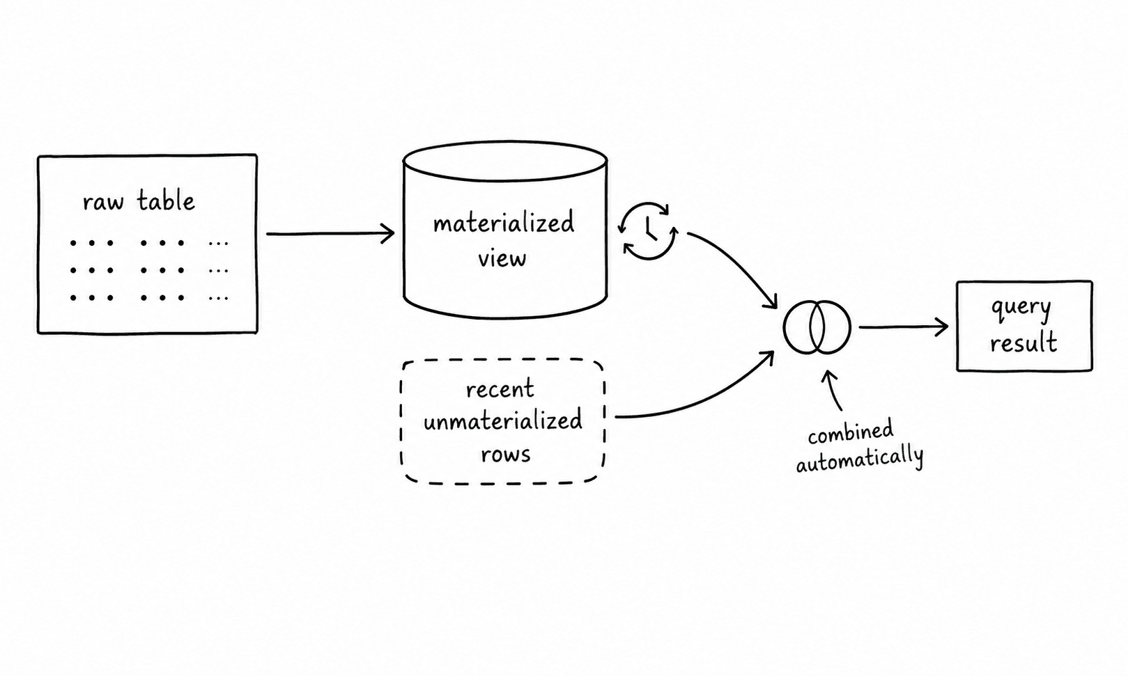
A continuous aggregate only reflects data as of its last refresh. Thanks to the end_offsetbuffer, it's always slightly behind the raw table. For an hourly view refreshing every hour, that could mean reports are up to an hour stale.
If a dashboard needs up-to-the-second numbers, enable real-time aggregation. Querying the continuous aggregate then transparently combines its materialized data with a live aggregation over the raw rows that haven't been materialized yet.
ALTER MATERIALIZED VIEW events_hourly SET (timescaledb.materialized_only = false);You get fast, pre-computed results for everything older than the last refresh and a small, cheap live aggregation for the recent sliver — combined into one result set without writing the union yourself.
Putting it together
Hypertable conversion, compression, continuous aggregates, refresh policies, and real-time aggregation turn a table that would otherwise need manual maintenance scripts and cron jobs into something that manages its own lifecycle. Old data compresses itself. Reporting views update themselves. Live dashboards stay accurate without querying the full raw table on every request.
None of it requires giving up the parts of Postgres you already know. It's still SELECT, GROUP BY, and standard SQL — TimescaleDB just handles the parts that get tedious and slow at scale, so you don't have to build that infrastructure by hand.